Collaborative Filtering

User-Based Approach

Unlike content-based methods that rely on item attributes or descriptions, collaborative filtering is driven purely by user behavior and interaction patterns. The central philosophy behind this approach is simple yet powerful: people who agreed in the past will likely agree again in the future. In other words, if two users have rated or interacted with many of the same items similarly, the system infers that their preferences are alike. Consequently, items liked or rated highly by one user are recommended to the other, even if they have never interacted with those items before.

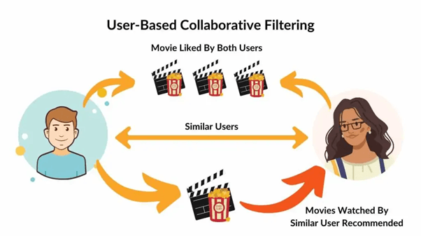
To achieve this, the system constructs a user–item interaction matrix, where each row represents a user and each column represents an item (e.g., movies, songs, or products). Missing values in this matrix—items not yet rated—are what the recommender tries to predict. The similarity between users is computed using statistical or distance-based measures like Cosine Similarity, Pearson Correlation, or Jaccard Index. These metrics help quantify how closely two users’ preferences align based on their rating patterns or behavioral overlaps.

For example, consider the following small dataset and similarity computation:

import numpy as np
from sklearn.metrics.pairwise import cosine_similarity
ratings = np.array([[5, 4, 0],
                   [3, 0, 4],
                   [0, 5, 5]])
user_similarity = cosine_similarity(ratings)
print(np.round(user_similarity, 2))

Here, each row represents a user and each column an item. The resulting similarity matrix quantifies how closely each pair of users’ tastes match. If User 1 and User 2 show a high similarity score, the system might recommend items that User 1 liked but User 2 hasn’t tried yet. Over time, as more data accumulates, the system refines these relationships, continuously improving recommendation accuracy.

User-based collaborative filtering is intuitive and easy to interpret, but it can struggle when the dataset becomes very large or sparse—meaning users have interacted with only a small fraction of items. Nevertheless, it remains a foundational technique and serves as the conceptual backbone for more advanced models like item-based filtering and matrix factorization, which we’ll explore next.

Item-Based Approach

The item-based collaborative filtering technique builds on the same foundation as the user-based approach but shifts the focus from users to items. Instead of finding similar users, this method identifies items that are similar based on user behavior patterns. The core intuition is that if two items are frequently liked or rated similarly by the same group of users, they are likely to be related. Therefore, if a user enjoys one item, the system can recommend the other, even if the user has never interacted with it before.

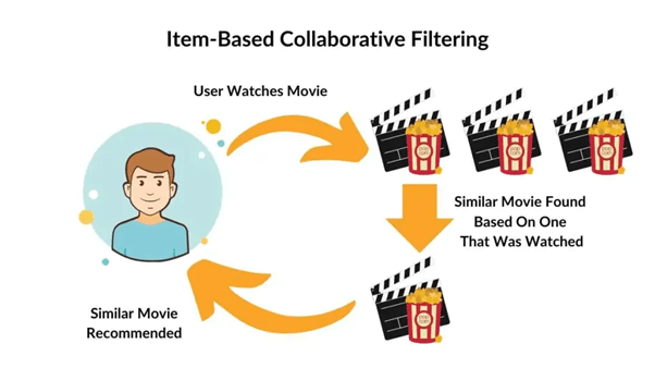
In practice, the algorithm constructs an item–item similarity matrix, where each cell represents how closely two items are related in terms of user ratings. The similarity is commonly measured using Cosine Similarity, Adjusted Cosine, or Pearson Correlation. For example, in a movie recommendation scenario, if users who liked Inception also tend to enjoy Interstellar, these two items will have a high similarity score. So, when a new user watches and likes Inception, the model confidently recommends Interstellar as the next suggestion.

Here’s a simple example to visualize the concept:

import numpy as np
from sklearn.metrics.pairwise import cosine_similarity
ratings = np.array([[5, 4, 0],
                   [3, 0, 4],
                   [0, 5, 5]])
item_similarity = cosine_similarity(ratings.T)
print(np.round(item_similarity, 2))

In this case, by transposing the ratings matrix, we shift the focus from users to items. The resulting similarity scores reveal which items have been rated similarly across users. If Item 1 and Item 3, for instance, share a high similarity value, the recommender system can use that insight to generate targeted recommendations.

One of the biggest strengths of item-based collaborative filtering is stability. While user preferences can change frequently, item characteristics and relationships tend to remain consistent. This makes item-based models more reliable and scalable for large systems like Amazon’s “Customers who bought this also bought” feature. However, as with any collaborative approach, it still faces challenges such as data sparsity and cold-start problems—issues that later hybrid or matrix-based models attempt to overcome.

Matrix Factorization using SVD

As datasets grow larger and sparser, traditional user-based and item-based collaborative filtering techniques begin to struggle. This is where Matrix Factorization (MF) comes into play — a powerful approach that reduces high-dimensional user–item interaction data into compact, meaningful representations. The goal of matrix factorization is to uncover the latent factors that drive user preferences and item characteristics, revealing hidden patterns that simple similarity measures can’t detect.

At its core, matrix factorization assumes that a user’s rating of an item is determined by the interaction between their respective latent feature vectors. These vectors capture abstract attributes — for example, in a movie domain, latent factors might represent genre affinity, mood, or storytelling style. Mathematically, the user–item rating matrix RRR (of size m×n) is decomposed into two smaller matrices:

U: the user-feature matrix (m×k), representing users in the latent factor space
V: the item-feature matrix (n×k), representing items in the same space

By multiplying U and V^T, we reconstruct an approximate version of RRR, filling in the missing entries with predicted ratings.

A popular method to achieve this decomposition is Singular Value Decomposition (SVD). SVD breaks down the rating matrix into three matrices U,Σ, V^T, where Σ contains singular values that indicate the importance of each latent feature. In practice, we can truncate these matrices to keep only the top k components, which reduces noise and captures the most significant underlying patterns.

Here’s a short implementation example:

import numpy as np
from numpy.linalg import svd
# User-Item rating matrix
R = np.array([[5, 4, 0],
             [3, 0, 4],
             [0, 5, 5]])
# Apply SVD
U, sigma, Vt = svd(R, full_matrices=False)
# Reconstruct with top k features
k = 2
R_approx = np.dot(U[:, :k], np.dot(np.diag(sigma[:k]), Vt[:k, :]))
print(np.round(R_approx, 2))

In this example, the missing ratings are estimated based on the learned latent features. By controlling the number of latent dimensions kkk, we balance between capturing sufficient complexity and avoiding overfitting.

Matrix factorization became widely popular after the Netflix Prize (2006), where it outperformed traditional techniques by a large margin. It enables more personalized and nuanced recommendations by capturing subtle relationships between users and items. However, it also requires careful tuning and can struggle with cold-start scenarios where no prior interaction data exists. Despite these challenges, matrix factorization remains a foundational concept in modern recommender systems, influencing advanced methods like deep learning and neural collaborative filtering.