


Your Success, Our Mission!
3000+ Careers Transformed.

Mathematical Foundations
Last Updated: 29th January, 2026Mathematical Foundations
Behind every powerful recommendation engine lies a solid mathematical backbone. This chapter explores the core mathematical concepts that drive personalization — from similarity measures and user-item matrices to latent factors and matrix factorization. You’ll gain the quantitative understanding necessary to make your models accurate, scalable, and interpretable. These foundations will help you transition from intuitive understanding to data-driven implementation in the later, model-building stages.
Similarity Measures (Cosine, Pearson, Jaccard)
Similarity measures help the system determine how alike two users or items are. They are critical in Collaborative Filtering to find neighbors or similar items.
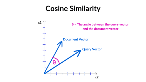
Cosine Similarity
Measures the angle between two vectors in a multidimensional space.
Ignore the magnitude; focus on the direction of preferences.
Formula:
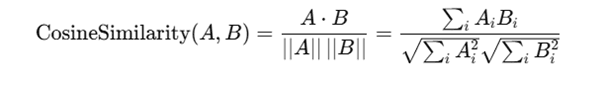
Range: -1 (opposite) to 1 (identical)
Python Example:
from sklearn.metrics.pairwise import cosine_similarity
import numpy as np
ratings = np.array([
   [5, 4, 0],
   [3, 0, 4]
])
similarity = cosine_similarity(ratings)
print(similarity)
Interpretation: Cosine similarity captures preference patterns even if users rate on different scales.
Pearson Correlation
Measures linear correlation between two users/items.
Accounts for differences in rating scale among users.
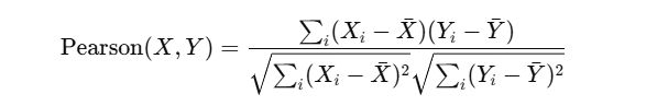
Range: -1 (inverse correlation), 0 (no correlation), 1 (perfect correlation)
Use Case: Better when users have different rating tendencies (e.g., one rates generously, one rates conservatively).
Jaccard Similarity
Measures overlap between two sets, often used for implicit feedback.
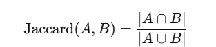
Works well for implicit feedback (clicks, purchases).
Range: 0 (no overlap) to 1 (complete overlap).
Example:
User1 bought {A, B, C}
User2 bought {B, C, D}
Jaccard similarity = 2 / 4 = 0.5
Ideal for binary interactions (clicked/not clicked, purchased/not purchased).
Key Insights:
Cosine → vector-based, ignores magnitude
Pearson → adjusts for user mean, ideal for rating scales
Jaccard → set-based, ideal for implicit data
Choosing the correct similarity measure is crucial depending on the type of data and business problem.
User-Item Matrix, Ratings, and Sparsity
User-Item Matrix (R)
Core representation of user interactions.
Rows = users, Columns = items, Values = explicit (ratings) or implicit (clicks, purchases)
Example Table:
| User | Movie A | Movie B | Movie C |
|---|---|---|---|
| U1 | 5 | 4 | ? |
| U2 | 3 | ? | 4 |
| U3 | ? | 5 | 5 |
Missing entries are the predictions the recommender must fill.
Sparsity in Real-World Systems
Real datasets are mostly sparse because:
- Users rate only a small fraction of items
- Many items are rarely interacted with
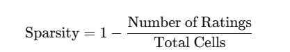
Sparsity rate formula:
High sparsity → difficult to compute reliable similarities
Handling Sparsity:
- Fill missing values with mean ratings
- Use matrix factorization to infer hidden preferences
- Use hybrid models combining content and collaborative methods
Python Example: User-Item Matrix
import pandas as pd
ratings = pd.DataFrame({
   'User': ['U1','U1','U2','U2','U3','U3'],
   'Movie': ['A','B','A','C','B','C'],
   'Rating': [5,4,3,4,5,5]
})
user_item_matrix = ratings.pivot_table(index='User', columns='Movie', values='Rating')
print(user_item_matrix)
Output:
| User | Movie A | Movie B | Movie C |
|---|---|---|---|
| U1 | 5 | 4 | ? |
| U2 | 3 | ? | 4 |
| U3 | ? | 5 | 5 |
Understanding Latent Factors and Matrix Factorization
Latent factors uncover hidden dimensions that explain why users like certain items.
Concept of Latent Factors
Hidden factors explain preferences not visible in raw data.
Example for movies:
Action vs Romance
Comedy vs Thriller
Popularity trend
Each user and item can be represented as vectors in latent space.
Matrix Factorization
Decomposes user-item matrix RRR into user matrix P and item matrix Q:

Where:
RRR = original ratings matrix
PPP = user latent factor matrix (users × factors)
QQQ = item latent factor matrix (items × factors)
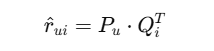
Predicted rating:
Optimization: Minimize squared error + regularization:
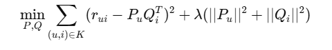
Where: K = observed ratings, λ\lambdaλ = regularization
Python Example: SVD with Surprise Library
from surprise import SVD, Dataset, Reader
from surprise.model_selection import train_test_split
import pandas as pd
ratings_dict = {'user_id': ['U1','U1','U2','U2','U3','U3'],
               'item_id': ['A','B','A','C','B','C'],
               'rating': [5,4,3,4,5,5]}
df = pd.DataFrame(ratings_dict)
reader = Reader(rating_scale=(1,5))
data = Dataset.load_from_df(df[['user_id','item_id','rating']], reader)
trainset, testset = train_test_split(data, test_size=0.3)
model = SVD()
model.fit(trainset)
pred = model.predict('U1','C')
print(pred.est)
SVD predicts missing ratings by learning latent factors.
Works well with sparse matrices and large datasets.
Key Insights:
Latent factors reveal hidden preferences of users and items.
Matrix factorization is highly effective for prediction.
Modern systems often use deep learning embeddings for richer representations.
Module 1: Introduction to Recommendation Systems
Top Tutorials
Related Articles
Made with in Bengaluru, India


- Courses
- Advanced Certification in Data Analytics & Gen AI Engineering
- Advanced Certification in Web Development & Gen AI Engineering
- MS in Computer Science: Machine Learning and Artificial Intelligence
- MS in Computer Science: Cloud Computing with AI System Design
- Professional Fellowship in Data Science and Agentic AI Engineering
- Professional Fellowship in Software Engineering with AI and DevOps
- Join AlmaBetter
- Sign Up
- Become A Coach
- Coach Login
- Policies
- Privacy Statement
- Terms of Use
- Contact Us
- admissions@almabetter.com
- 08046008400
- Official Address
- 4th floor, 133/2, Janardhan Towers, Residency Road, Bengaluru, Karnataka, 560025
- Communication Address
- Follow Us

© 2026 AlmaBetter